3 Mapping Carl Nielsens Works
This notebook is about analyzing the musical works of Carl Nielsen, by using digital methods.R is going to be used for examining: - Which author has Carl Nielsen composed most works for - Where have Carl Nielsens Works been performed? - Which titles were performed in which countries
The overall area of interest is the Danish composer Carl Nielsen’s works. These works have been collected and organised into the platform Catalogue of Carl Nielsen’s Works by the former Danish Centre for Music Editing at the Royal Danish Library. The material used in this workshop is data extracted from the raw data used in the catalogue mentioned above. The data has then been organised in the R-data format in order to make this workshop more about analysing the data rather than parsing it.
The data used on the platform Catalogue of Carl Nielsen’s Works is availabe in raw xml format here: Download-site raw xml data for Carl Nielsen’s Works. The catalogue uses the MEI xml format, designed to encode notated music as well as comprehensive musical metadata. The Carl Nielsen catalogue uses only the metadata part; the notated music (scores) are not included in the encoding. The MEI standard is developed and maintained by the Music Encoding Initiative.
3.1 Loading Libraries
The dataset is processed in the software programme R, offering various methods for statistical analysis and graphic representation of the results. In R, one works with packages each adding numerous functionalities to the core functions of R. In this example, the relevant packages are:
3.2 Load data
The code below reads data from a RDS file named “cnw_dataframe.rds” and stores it in a variable called cnw.A RDS-file is a single-object R data file used to save and load one R object (like a model or dataframe).
3.4 Which city/place has seen most performances of Carl Nielsen Works?
For now we’ll just look at a single work:
## # A tibble: 1 × 17
##   file       title_da title_en title_sub_da title_sub_en composer author creation classification_1 classification_2 classification_3
##   <chr>      <chr>    <chr>    <chr>        <chr>        <chr>    <chr>  <chr>    <chr>            <chr>            <chr>
## 1 ../data-c… Saul og… Saul an… Opera i fir… Opera in Fo… Carl Ni… Einar… 1899–19… Stage music      Opera            <NA>
## # ℹ 6 more variables: classification_4 <chr>, classification_5 <chr>, classification_6 <chr>, history <chr>, performances <list>,
## #   music <list>
We see that the row under performances holds a “tibble”, which is a dataframe. This dataframe contains all the performances of Saul and David, but we cant count how many because it is in a dataframe within a row. But we can unpack this dataframe while retaining all the other information:
## # A tibble: 112 × 23
##    file      title_da title_en title_sub_da title_sub_en composer author creation classification_1 classification_2 classification_3
##    <chr>     <chr>    <chr>    <chr>        <chr>        <chr>    <chr>  <chr>    <chr>            <chr>            <chr>
##  1 ../data-… Saul og… Saul an… Opera i fir… Opera in Fo… Carl Ni… Einar… 1899–19… Stage music      Opera            <NA>
##  2 ../data-… Saul og… Saul an… Opera i fir… Opera in Fo… Carl Ni… Einar… 1899–19… Stage music      Opera            <NA>
##  3 ../data-… Saul og… Saul an… Opera i fir… Opera in Fo… Carl Ni… Einar… 1899–19… Stage music      Opera            <NA>
##  4 ../data-… Saul og… Saul an… Opera i fir… Opera in Fo… Carl Ni… Einar… 1899–19… Stage music      Opera            <NA>
##  5 ../data-… Saul og… Saul an… Opera i fir… Opera in Fo… Carl Ni… Einar… 1899–19… Stage music      Opera            <NA>
##  6 ../data-… Saul og… Saul an… Opera i fir… Opera in Fo… Carl Ni… Einar… 1899–19… Stage music      Opera            <NA>
##  7 ../data-… Saul og… Saul an… Opera i fir… Opera in Fo… Carl Ni… Einar… 1899–19… Stage music      Opera            <NA>
##  8 ../data-… Saul og… Saul an… Opera i fir… Opera in Fo… Carl Ni… Einar… 1899–19… Stage music      Opera            <NA>
##  9 ../data-… Saul og… Saul an… Opera i fir… Opera in Fo… Carl Ni… Einar… 1899–19… Stage music      Opera            <NA>
## 10 ../data-… Saul og… Saul an… Opera i fir… Opera in Fo… Carl Ni… Einar… 1899–19… Stage music      Opera            <NA>
## # ℹ 102 more rows
## # ℹ 12 more variables: classification_4 <chr>, classification_5 <chr>, classification_6 <chr>, history <chr>, isodate <chr>,
## #   startdate <chr>, enddate <chr>, place <chr>, venue <chr>, ensemble <chr>, conductor <chr>, music <list>
There is 112 performances of Saul and David. But this is just for one work. We do the same for the entire dataset and save it to a new data frame, since we are changing dramatically on the form of of the data. We’re making the shift from having one work pr. row to have one performances of a work pr. row:
Since all the other data have been retained for each performances we can now count to see which work has been performened the most:
## # A tibble: 252 × 2
##    title_da                                                                                        n
##    <chr>                                                                                       <int>
##  1 "Maskarade"                                                                                   602
##  2 "Musik til Adam Oehlenschlägers skuespil \"Aladdin eller Den forunderlige Lampe\", opus 34"   211
##  3 "Jeg bærer med Smil min Byrde"                                                                204
##  4 "Jens Vejmand, opus 21.3"                                                                     155
##  5 "Æbleblomst, opus 10.1"                                                                       121
##  6 "Saul og David"                                                                               112
##  7 "Sang bag Ploven, opus 10.4"                                                                   96
##  8 "Silkesko over gylden Læst!, opus 6.3"                                                         96
##  9 "Musik til Helge Rodes skuespil \"Moderen\", opus 41"                                          92
## 10 "Suite for strygeorkester, opus 1"                                                             87
## # ℹ 242 more rows
Following the same logic we can also examine which city has seen the most performances:
## # A tibble: 241 × 2
##    place            n
##    <chr>        <int>
##  1 "Copenhagen"  2950
##  2 "Gothenburg"   112
##  3 "Stockholm"    111
##  4 "Odense"        92
##  5 "Aarhus"        88
##  6 ""              55
##  7 "Berlin"        43
##  8 "Aalborg"       42
##  9 "Oslo"          42
## 10 "Ryslinge"      41
## # ℹ 231 more rows
Copenhagen is out of proportions - lets filter it out for a nice visualisation:
cnw_performances %>%
filter(place != "") %>%
filter(place != "Copenhagen") %>%
count(place, sort = TRUE) %>%
slice_max(n, n = 15) %>%
mutate(place = reorder(place, n)) %>%
ggplot(aes(x = place, y = n)) +
geom_col(fill = "lightblue") +
coord_flip() +
labs(
title = "Performances of Carl Nielsen works outside of Copenhagen",
subtitle = "- dispersed on cities",
caption = "Data from Catalogue of Carl Nielsen's Works (CNW)",
x = "City",
y = "Count of performances"
) 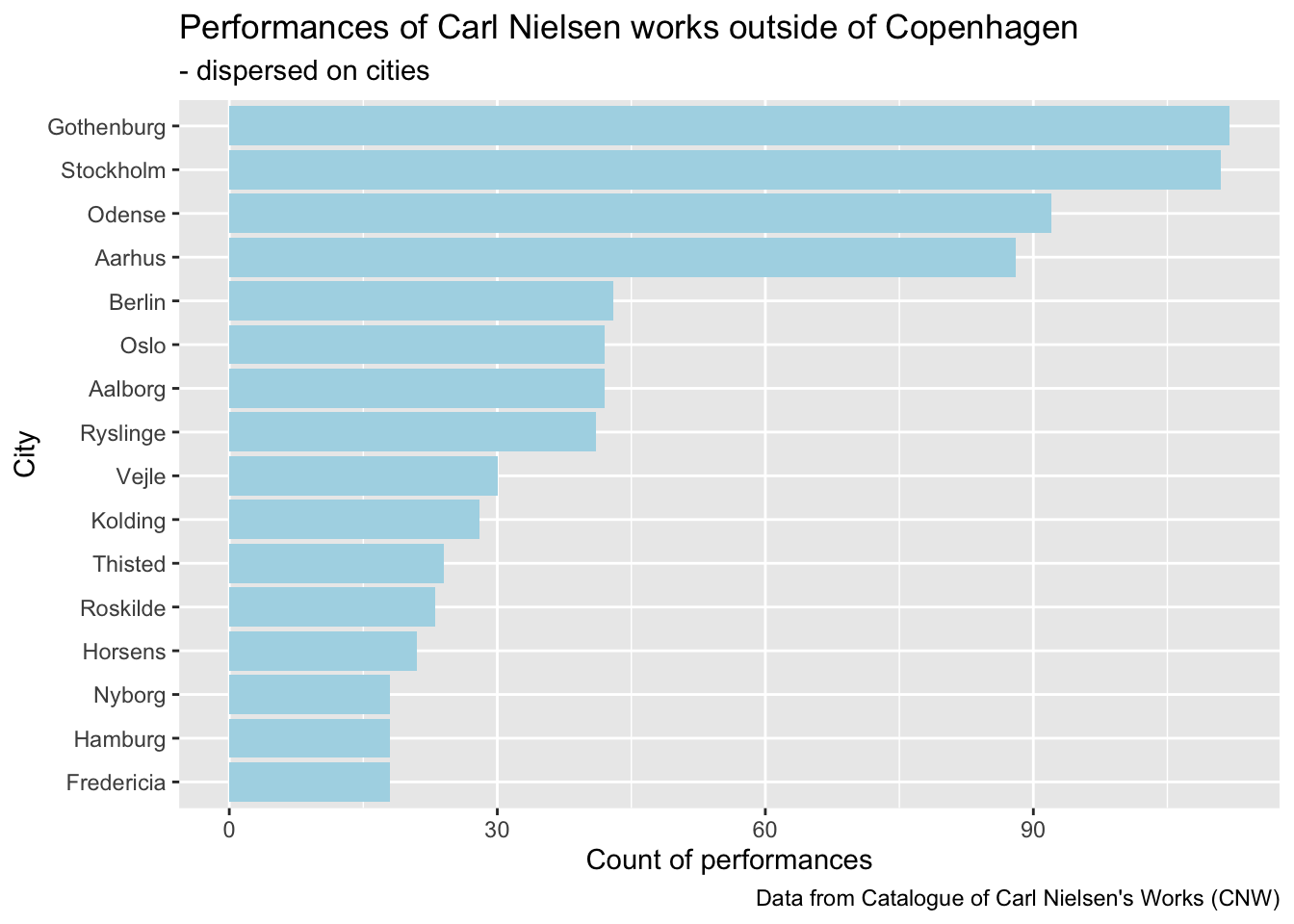 This code filters and counts the top 15 non-Copenhagen cities using tidyverse pipes, and the shift to visualization is clearly marked when the syntax switches from %>% to +, which signals moving from data-wrangling logic into ggplot layer-building logic.
3.5 Which titles in which countries?
Load geographical data about cities with 3 or more performances of Carl Nielsen Works:
cnw_cities <- readRDS(url("https://raw.githubusercontent.com/maxodsbjerg/MappingCarlNielsensWorks/refs/heads/main/data-output/20241020_cnw_performances_geographical_information.rds"))Add the geographical data to the performances data frame:
Dispersions of performances on country:
## # A tibble: 20 × 2
##    country             n
##    <chr>           <int>
##  1 Danmark          3842
##  2 Sverige           242
##  3 Deutschland       120
##  4 Norge              49
##  5 Nederland          15
##  6 France             14
##  7 Suomi / Finland    13
##  8 Polska              8
##  9 United Kingdom      8
## 10 Česko               8
## 11 Österreich          7
## 12 Magyarország        6
## 13 United States       6
## 14 Hrvatska            2
## 15 Italia              2
## 16 România             2
## 17 日本                2
## 18 España              1
## 19 Kenya               1
## 20 Latvija             1
Which titles has been performed the most in Denmark:
## # A tibble: 251 × 2
##    title_da                                                                                        n
##    <chr>                                                                                       <int>
##  1 "Maskarade"                                                                                   512
##  2 "Jeg bærer med Smil min Byrde"                                                                195
##  3 "Musik til Adam Oehlenschlägers skuespil \"Aladdin eller Den forunderlige Lampe\", opus 34"   157
##  4 "Jens Vejmand, opus 21.3"                                                                     149
##  5 "Æbleblomst, opus 10.1"                                                                       117
##  6 "Sang bag Ploven, opus 10.4"                                                                   89
##  7 "Musik til Helge Rodes skuespil \"Moderen\", opus 41"                                          87
##  8 "Silkesko over gylden Læst!, opus 6.3"                                                         87
##  9 "Sænk kun dit Hoved, du Blomst, opus 21.4"                                                     76
## 10 "Saul og David"                                                                                75
## # ℹ 241 more rows