Bigram Analysis of Trykkefrihedens Skrifter#
Script Summary#
This notebook performs bigram (word pair) analysis on Trykkefrihedens Skrifter in Python, inspired by the R workflow. Bigram analysis identifies frequently co-occurring word pairs to reveal linguistic patterns and phrase structures in historical Danish texts.
Steps:
Load the structured dataset and project-specific stopwords
Create bigrams (word pairs) for each text in the dataset
Count the frequency of each bigram across the corpus
Filter out bigrams containing stopwords to focus on meaningful word combinations
Search for specific bigrams matching patterns (e.g., words starting with ‘gud’)
Visualize frequent bigrams as network graphs showing word relationships
Export results to CSV files and save network visualizations
Outputs: Bigram frequency tables, filtered bigram results, pattern-matched bigrams, network graph visualizations, and CSV files for further analysis.
Install and Import Dependencies#
If you’re missing any packages, uncomment and run the pip cell below.
# !pip install pandas numpy nltk matplotlib seaborn networkx

import pandas as pd
import numpy as np
import re
import nltk
from nltk.corpus import stopwords
import matplotlib.pyplot as plt
import seaborn as sns
import networkx as nx

nltk.download('punkt')
nltk.download('stopwords')
[nltk_data] Downloading package punkt to
[nltk_data]     C:\Users\lakj\AppData\Roaming\nltk_data...
[nltk_data]   Package punkt is already up-to-date!
[nltk_data] Downloading package stopwords to
[nltk_data]     C:\Users\lakj\AppData\Roaming\nltk_data...
[nltk_data]   Package stopwords is already up-to-date!
True
Load Data#
Check your data files: You need the main text data and project-specific stopwords as csv files.
tfs_structured.csv— Main text datatfs_stopord.csv— Project-specific stopwords
You can find them in the corresponding repository: kb-dk/cultural-heritage-data-guides-Python
Or you can load them through these links:
https://raw.githubusercontent.com/maxodsbjerg/TextMiningTFS/refs/heads/main/data/tfs_structured.csv
https://raw.githubusercontent.com/maxodsbjerg/TextMiningTFS/refs/heads/main/data/tfs_stopord.csv
Here we load the .csv files from our project folder.
The Data Structure in tfs_structured.csv is:
refnr: Reference numberrække: Series numberbind: Volume numberside: Page numbercontent: Text content
With the data in the right folder we load the main data and stopwords from CSV files.
main_data_path = 'tfs_structured.csv'
stopwords_path = 'tfs_stopord.csv'

try:
    tfs = pd.read_csv(main_data_path)
    print(f'Data loaded. Shape: {tfs.shape}')
except FileNotFoundError:
    print(f'File not found: {main_data_path}')
    tfs = None

try:
    stopord_tfs = pd.read_csv(stopwords_path)['word'].astype(str).str.lower().tolist()
    print(f'Loaded {len(stopord_tfs)} project-specific stopwords.')
except Exception as e:
    print(f'Could not load project-specific stopwords: {e}')
    stopord_tfs = []

# Optional extra stopwords list from URL (can be added if desired)
# stopord_url = "https://gist.githubusercontent.com/maxodsbjerg/4d1e3b1081ebba53a8d2c3aae2a1a070/raw/e1f63b4c81c15bb58a54a2f94673c97d75fe6a74/stopord_18.csv"
# stopord_extra = pd.read_csv(stopord_url)['word'].astype(str).str.lower().tolist()
# stopord_tfs += stopord_extra
Data loaded. Shape: (28133, 14)
Loaded 60 project-specific stopwords.
Formation of Bigrams#
We create bigrams (word pairs) for each text.
def regex_tokenize(text):
    # Simple tokenization, can be extended if needed
    return re.findall(r'\b\S+\b', str(text).lower())

def make_bigrams(tokens):
    return [(tokens[i], tokens[i+1]) for i in range(len(tokens)-1)]

# Create bigrams for all rows
if tfs is not None:
    bigrams_list = []
    for idx, row in tfs.iterrows():
        tokens = regex_tokenize(row['content'])
        bigrams = make_bigrams(tokens)
        for bg in bigrams:
            bigrams_list.append({'refnr': row.get('refnr', idx),
                                 'række': row.get('række', None),
                                 'bind': row.get('bind', None),
                                 'side': row.get('side', None),
                                 'word1': bg[0],
                                 'word2': bg[1]})

    tfs_bigrams = pd.DataFrame(bigrams_list)
    print(f'Number of bigrams: {len(tfs_bigrams)}')
    display(tfs_bigrams.head())
else:
    print('Data not loaded. Please ensure tfs_structured.csv is available.')
    tfs_bigrams = pd.DataFrame()
Number of bigrams: 4402472
| refnr | række | bind | side | word1 | word2 | |
|---|---|---|---|---|---|---|
| 0 | 1.1.1 | 1 | 1 | 1 | philopatreias | trende |
| 1 | 1.1.1 | 1 | 1 | 1 | trende | anmærkninger |
| 2 | 1.1.1 | 1 | 1 | 1 | anmærkninger | i |
| 3 | 1.1.1 | 1 | 1 | 1 | i | om |
| 4 | 1.1.1 | 1 | 1 | 1 | om | de |
Count Bigrams#
We count the frequency of each bigram (word pair).
bigram_counts = tfs_bigrams.groupby(['word1', 'word2']).size().reset_index(name='count')
bigram_counts = bigram_counts.sort_values('count', ascending=False)
display(bigram_counts.head(20))
| word1 | word2 | count | |
|---|---|---|---|
| 1417738 | til | at | 10099 |
| 335398 | det | er | 6434 |
| 507506 | for | at | 6155 |
| 130779 | at | de | 5393 |
| 444015 | er | det | 3924 |
| 132588 | at | han | 3605 |
| 759583 | i | det | 3584 |
| 759543 | i | den | 3010 |
| 759924 | i | en | 3003 |
| 130867 | at | det | 2853 |
| 1071406 | og | at | 2728 |
| 1328585 | som | de | 2636 |
| 1074505 | og | det | 2563 |
| 130821 | at | den | 2497 |
| 61524 | af | de | 2487 |
| 1328912 | som | en | 2445 |
| 1081091 | og | i | 2432 |
| 137823 | at | være | 2378 |
| 133386 | at | jeg | 2354 |
| 1074337 | og | de | 2252 |
Remove Bigrams Where One of the Words is a Stopword#
We remove bigrams where either word1 or word2 is a stopword (Danish, German, or project-specific).
stopord_da = set(stopwords.words('danish'))
stopord_de = set(stopwords.words('german'))
stopord_all = stopord_da | stopord_de | set(stopord_tfs)

bigrams_filtered = tfs_bigrams[
    (~tfs_bigrams['word1'].isin(stopord_all)) &
    (~tfs_bigrams['word2'].isin(stopord_all))
]
print(f'Number of bigrams after stopword filtering: {len(bigrams_filtered)}')
Number of bigrams after stopword filtering: 966952
Count Filtered Bigrams#
We now count bigrams without stopwords.
bigram_counts_filtered = bigrams_filtered.groupby(['word1', 'word2']).size().reset_index(name='count')
bigram_counts_filtered = bigram_counts_filtered.sort_values('count', ascending=False)
display(bigram_counts_filtered.head(20))
| word1 | word2 | count | |
|---|---|---|---|
| 358413 | kiøbenhavn | 1771 | 477 |
| 552523 | skilling | stor | 353 |
| 9418 | 1771 | trykt | 318 |
| 560772 | slet | intet | 305 |
| 358686 | kiøbenhavn | trykt | 275 |
| 9615 | 1772 | trykt | 272 |
| 524686 | s | v | 266 |
| 461193 | o | s | 266 |
| 340844 | intet | andet | 262 |
| 381451 | lang | tid | 251 |
| 358414 | kiøbenhavn | 1772 | 228 |
| 368694 | kort | tid | 220 |
| 364293 | kong | christian | 218 |
| 200040 | findes | tilkiøbs | 207 |
| 191 | 1 | ark | 206 |
| 349143 | junior | philopatreias | 200 |
| 839 | 1/2 | ark | 195 |
| 392811 | ligesaa | lidet | 182 |
| 23815 | 4 | skilling | 176 |
| 581354 | stor | 1 | 175 |
Search for Specific Bigrams (e.g., where word2 matches a pattern)#
We can filter bigrams where word2 matches a specific pattern, e.g., words starting with ‘gud’.
pattern = r'\bgud[a-zæø]*'
match_bigrams = bigrams_filtered[bigrams_filtered['word2'].str.contains(pattern, regex=True)]
match_counts = match_bigrams.groupby(['word1', 'word2']).size().reset_index(name='count')
match_counts = match_counts.sort_values('count', ascending=False)
display(match_counts.head(20))
| word1 | word2 | count | |
|---|---|---|---|
| 1523 | o | gud | 95 |
| 1145 | imod | gud | 83 |
| 1935 | store | gud | 47 |
| 2011 | takke | gud | 38 |
| 816 | frygte | gud | 35 |
| 993 | herre | gud | 32 |
| 1195 | jordens | guder | 31 |
| 1148 | imod | guds | 31 |
| 913 | gode | gud | 29 |
| 1791 | sande | gud | 28 |
| 1794 | sande | guds | 21 |
| 821 | frygter | gud | 21 |
| 531 | elske | gud | 21 |
| 2042 | tiene | gud | 19 |
| 241 | bede | gud | 19 |
| 1217 | kiende | gud | 18 |
| 1706 | retfærdige | gud | 17 |
| 159 | almægtige | gud | 16 |
| 937 | gudernes | gud | 16 |
| 1787 | sand | gudsfrygt | 16 |
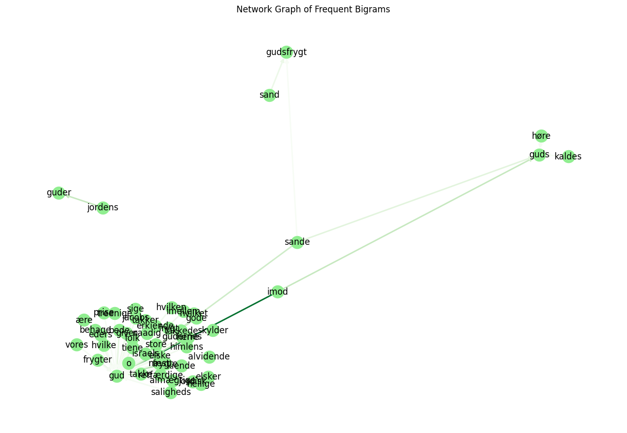
Visualization as Network Graph#
We can visualize the most frequent bigrams as a network graph.
# Select bigrams that occur more than e.g., 8 times
threshold = 8
graph_data = match_counts[match_counts['count'] > threshold]

G = nx.DiGraph()
for _, row in graph_data.iterrows():
    G.add_edge(row['word1'], row['word2'], weight=row['count'])

plt.figure(figsize=(12, 8))
pos = nx.spring_layout(G, k=0.5)
edges = G.edges()
weights = [G[u][v]['weight'] for u,v in edges]
nx.draw(G, pos, with_labels=True, node_color='lightgreen', edge_color=weights, width=2.0, edge_cmap=plt.cm.Greens, arrows=True)
plt.title('Network Graph of Frequent Bigrams')
plt.show()
Save Graph and Results#
You can save the graph and results as CSV files.
bigram_counts_filtered.to_csv('results_bigrams_filtered.csv', index=False)
match_counts.to_csv('results_bigrams_match.csv', index=False)
plt.savefig('graphics/bigram_network.png', bbox_inches='tight', dpi=150)
print('Results and graph saved.')
Results and graph saved.
<Figure size 640x480 with 0 Axes>
Other studies#
The bigram analysis of Trykkefrihedens Skrifter can be extended with several complementary approaches:
Expand pattern matching to explore other semantic domains (e.g., political terms, social concepts, religious language) and identify distinctive phrase patterns.
Analyze temporal changes in bigram usage by comparing frequent word pairs across different publication periods.
Investigate trigram and n-gram patterns to explore longer phrase structures and multi-word expressions.
Apply network analysis techniques to identify central nodes and communities in the bigram network.
Compare bigram patterns with other historical Danish text collections to identify genre-specific or period-specific linguistic features.
Explore the relationship between bigram frequency and semantic coherence to identify meaningful versus coincidental co-occurrences.
Analyze bigram patterns in specific volumes or series to identify thematic or stylistic variations.
Integrate bigram analysis with topic modeling to understand how word pairs contribute to broader thematic structures.