Explore the Copenhagen Diplomatarium dataset (Københavns Diplomatarium)#
Script Summary#
This notebook explores the Copenhagen Diplomatarium dataset, which contains historical documents from medieval and early modern Denmark. The analysis focuses on text mining techniques to understand language patterns, word frequencies, and linguistic features of historical Danish texts.
Steps:
Load the Copenhagen Diplomatarium dataset from a CSV file
Explore the dataset structure and time period coverage
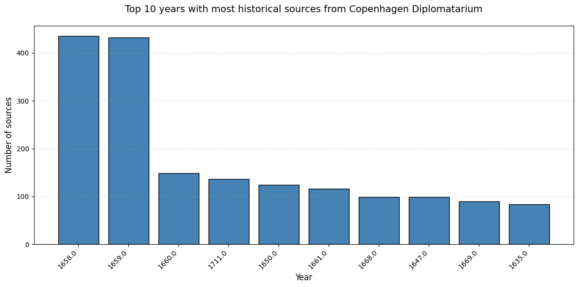
Analyze the distribution of sources across different years
Visualize the top years with the most historical sources
Perform word frequency analysis for a specific year (1658)
Visualize the most common words from selected periods
Analyze word collocations (bigrams and trigrams) across the entire corpus
Perform concordance analysis to examine keyword contexts
Outputs: Word frequency distributions, collocation analysis results, concordance tables, and visualizations revealing linguistic patterns in historical Danish documents.
Dataset: To download the dataset follow go to the Library’s Open Access Repository.
Import Libraries#
Import the required libraries for data manipulation, text processing, and visualization. NLTK resources are downloaded if not already present.
import pandas as pd
import re
import nltk
from nltk.probability import FreqDist
from nltk.collocations import BigramCollocationFinder, TrigramCollocationFinder
from nltk.metrics import BigramAssocMeasures, TrigramAssocMeasures
from nltk.text import Text
import matplotlib.pyplot as plt
# Ensure the required NLTK resources are downloaded
nltk.download('punkt')  # Optional if you haven't already downloaded
[nltk_data] Downloading package punkt to
[nltk_data]     C:\Users\lakj\AppData\Roaming\nltk_data...
[nltk_data]   Package punkt is already up-to-date!
True
Load the Dataset#
Load the Copenhagen Diplomatarium dataset from a CSV file.
df = pd.read_csv('kd_std.csv')
Explore the Dataset Structure#
Display the column names to understand the dataset structure.
df.columns
Index(['volume', 'page', 'number', 'date', 'year_std', 'month_std', 'day_std',
       'date_std', 'summary', 'note', 'main_content', 'file_name'],
      dtype='object')
Time Period Analysis#
Display the time range covered by the dataset, showing the oldest and most recent sources.
# Time period
print (f"The oldest source is from: {df['year_std'].min()}")
print (f"The most recent source is from: {df['year_std'].max()}")
The oldest source is from: 1177.0
The most recent source is from: 1728.0
Count Sources by Year#
Count the number of sources per year and prepare the data for visualization.
year_count = df['year_std'].value_counts()\
                            .to_frame()\
                            .head(10)\
                            .reset_index()
Visualize Top Years#
Create a bar chart showing the top 10 years with the most historical sources.
# Bar plot of the 10 most frequent years
plt.figure(figsize=(12, 6))
plt.bar(year_count['year_std'].astype(str), year_count['count'], color='steelblue', edgecolor='black')
plt.xlabel('Year', fontsize=12)
plt.ylabel('Number of sources', fontsize=12)
plt.title('Top 10 years with most historical sources from Copenhagen Diplomatarium', fontsize=14, pad=20)
plt.xticks(rotation=45, ha='right')
plt.grid(axis='y', alpha=0.3, linestyle='--')
plt.tight_layout()
plt.show()
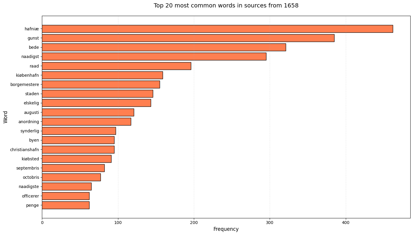
Word Frequency Analysis for Year 1658#
Extract and clean text from sources dated 1658, remove stopwords, and calculate word frequencies. This analysis focuses on a specific year to examine the language and terminology used during that period.
whole_1658 = ' '.join(df[df['year_std']==1658]['main_content'].to_list()).lower()
_clean_whole_1658 = ' '.join(re.findall(r'\b\S+\b', whole_1658))
_clean_whole_1658 = re.sub(r'\d+',' ', _clean_whole_1658)
_clean_whole_1658 = re.sub(r'\s+',' ', _clean_whole_1658)
_clean_whole_1658_wordlist = _clean_whole_1658.split()
with open('kd_stopwords.txt', 'r', encoding='utf-8') as f:
    stopword_list = f.read().split('\n')

clean_whole_1658_wordlist_wo_stopwords = [i for i in _clean_whole_1658_wordlist if i not in stopword_list]

freq_dist_1658 = FreqDist(clean_whole_1658_wordlist_wo_stopwords)

# Optional: To see the most common words
print(freq_dist_1658.most_common(20))
[('hafniæ', 462), ('gunst', 385), ('bede', 321), ('naadigst', 295), ('raad', 196), ('kiøbenhafn', 159), ('borgemestere', 155), ('staden', 146), ('elskelig', 143), ('augusti', 121), ('anordning', 117), ('synderlig', 97), ('byen', 95), ('christianshafn', 95), ('kiøbsted', 91), ('septembris', 82), ('octobris', 77), ('naadigste', 65), ('officerer', 62), ('penge', 62)]
Visualize Word Frequencies#
Create a horizontal bar chart displaying the top 20 most common words from sources dated 1658.
# Visualization of common words from the year 1658
top_words = freq_dist_1658.most_common(20)
words = [word for word, freq in top_words]
frequencies = [freq for word, freq in top_words]

plt.figure(figsize=(14, 8))
plt.barh(words, frequencies, color='coral', edgecolor='black')
plt.xlabel('Frequency', fontsize=12)
plt.ylabel('Word', fontsize=12)
plt.title('Top 20 most common words in sources from 1658', fontsize=14, pad=20)
plt.gca().invert_yaxis()  # Most frequent words at top
plt.grid(axis='x', alpha=0.3, linestyle='--')
plt.tight_layout()
plt.show()
Collocation Analysis#
Analyze word collocations (frequently co-occurring word pairs and triplets) across the entire corpus. Collocations reveal common phrases and linguistic patterns in the historical texts. The analysis uses Pointwise Mutual Information (PMI) to identify meaningful word combinations.
# NLTK collocation tool
whole_text_corpus = ' '.join(df['main_content'].astype(str))

# Clean the text
_clean_corpus = ' '.join(re.findall(r'\b\S+\b', whole_text_corpus))
_clean_corpus = re.sub(r'\d+', ' ', _clean_corpus)
clean_corpus = re.sub(r'\s+', ' ', _clean_corpus)

# Tokenize
tokens_clean = clean_corpus.split()

# Remove stopwords
with open('kd_stopwords.txt', 'r', encoding='utf-8') as f:
    stopword_list = f.read().split('\n')

# Find bigram collocations (2-word phrases)
bigram_finder = BigramCollocationFinder.from_words(tokens_clean)
bigram_finder.apply_freq_filter(3)  # Minimum 3 occurrences

print("=" * 60)
print("TOP 20 BIGRAM COLLOCATIONS (2-word phrases)")
print("=" * 60)
bigram_measures = BigramAssocMeasures()
top_bigrams = bigram_finder.nbest(bigram_measures.pmi, 20)  # PMI = Pointwise Mutual Information
for i, (word1, word2) in enumerate(top_bigrams, 1):
    freq = bigram_finder.ngram_fd[(word1, word2)]
    print(f"{i:2d}. '{word1} {word2}' (frequency: {freq})")

print("\n" + "=" * 60)
print("TOP 20 TRIGRAM COLLOCATIONS (3-word phrases)")
print("=" * 60)
# Find trigram collocations (3-word phrases)
trigram_finder = TrigramCollocationFinder.from_words(tokens_clean)
trigram_finder.apply_freq_filter(2)  # Minimum 2 occurrences

trigram_measures = TrigramAssocMeasures()
top_trigrams = trigram_finder.nbest(trigram_measures.pmi, 20)
for i, (word1, word2, word3) in enumerate(top_trigrams, 1):
    freq = trigram_finder.ngram_fd[(word1, word2, word3)]
    print(f"{i:2d}. '{word1} {word2} {word3}' (frequency: {freq})")
============================================================
TOP 20 BIGRAM COLLOCATIONS (2-word phrases)
============================================================
 1. 'Blandt Betingelserne' (frequency: 3)
 2. 'Botulphus Awæsson' (frequency: 3)
 3. 'Clementt Thettert' (frequency: 3)
 4. 'Ludolph Ringelman' (frequency: 3)
 5. 'Swers trommetters' (frequency: 3)
 6. 'Wigislef Walbu' (frequency: 3)
 7. 'Wilhelmus Toppius' (frequency: 3)
 8. 'mandtallers forfatning' (frequency: 3)
 9. 'ponerentur nutrirentur' (frequency: 3)
10. 'quintis feriis' (frequency: 3)
11. 'silentium imponendo' (frequency: 3)
12. 'udregninger mandtallers' (frequency: 3)
13. 'validius opitulantibus' (frequency: 3)
14. 'vasallis bondonibus' (frequency: 3)
15. 'Cice Oleffs' (frequency: 3)
16. 'Ciitzæ Tidickes' (frequency: 4)
17. 'Floritz Reinholtsen' (frequency: 3)
18. 'Gertridh Brandz' (frequency: 3)
19. 'Gotlob Skøn' (frequency: 3)
20. 'Hille Grauestens' (frequency: 3)

============================================================
TOP 20 TRIGRAM COLLOCATIONS (3-word phrases)
============================================================
 1. 'Cameracensi Tornacensi Morinensi' (frequency: 2)
 2. 'Coloniensi Treuerensi Saltzburgensi' (frequency: 2)
 3. 'Limfioren Steffuens herrith' (frequency: 2)
 4. 'Morinensi Attrebatensi Caminensi' (frequency: 2)
 5. 'Saltzburgensi Bremensi Bisuntinensi' (frequency: 2)
 6. 'Tornacensi Morinensi Attrebatensi' (frequency: 2)
 7. 'Treuerensi Saltzburgensi Bremensi' (frequency: 2)
 8. 'arckeliett prouiantthusett bryggerhusett' (frequency: 2)
 9. 'armaturas jocalia vesturas' (frequency: 2)
10. 'ciuitatenses solotenus prostratum' (frequency: 2)
11. 'ewren kunfftigen successorn' (frequency: 2)
12. 'nostræ Novi Castri' (frequency: 2)
13. 'prolixo languore infirmatur' (frequency: 2)
14. 'Archeliett Prouianthusitt Bryggerhusitt' (frequency: 2)
15. 'Janvario Aprili Julio' (frequency: 2)
16. 'Stoltzenborg Prolvitz Blankensee' (frequency: 2)
17. 'aliosque calices argenteos' (frequency: 2)
18. 'brott dauon gebackket' (frequency: 2)
19. 'consultandis moram trahere' (frequency: 2)
20. 'decreta exemptiones relaxationes' (frequency: 2)
Concordance Analysis#
Use NLTK’s concordance tool to find and display all contexts where a specific keyword appears. This allows examination of how a word is used in different contexts throughout the corpus. The example searches for “christianshafn” and displays surrounding text for each occurrence.
# NLTK Concordance tool - show all contexts for "christianshafn"

# Create full text corpus
whole_corpus = ' '.join(df['main_content'].astype(str).tolist()).lower()

# Light cleaning - keep punctuation for better context
clean_corpus_conc = re.sub(r'\s+', ' ', whole_corpus)

# Tokenize (split into words)
tokens = nltk.word_tokenize(clean_corpus_conc)

# Create NLTK Text object
text = nltk.Text(tokens)

print("=" * 80)
print("CONCORDANCE FOR 'christianshafn' - Shows context around each occurrence")
print("=" * 80)
print()

# Display concordance - set width and lines
text.concordance('christianshafn', width=70, lines=20)

print("\n" + "=" * 80)
print("STATISTICS")
print("=" * 80)
christianshafn_count = tokens.count('christianshafn')
print(f"Total number of occurrences of 'christianshafn': {christianshafn_count}")
print(f"Total number of tokens in corpus: {len(tokens):,}")
print(f"Frequency: {christianshafn_count/len(tokens)*100:.4f}%")
================================================================================
CONCORDANCE FOR 'christianshafn' - Shows context around each occurrence
================================================================================
Displaying 20 of 742 matches:
ppe , møller oc brygger paa christianshafn , en weyermølle , bebois af
 qv . tyck . herforuden ved christianshafn . 1. svend nielsen møller e
rin en platz i wor kiøbsted christianshafn och madtz pedersen nu sig i
børsen eller i wor kiøbstad christianshafn varene imod recessenn opleg
ster oc raad i vor kiøbsted christianshafn , at deris encher effter de
 , indvaaner i vor kiøbsted christianshafn , oc hans arfvinger en wor
660. borgemestere oc raad i christianshafn fich bref paa steen i st. a
ll mestere eller dennem udi christianshafn , uden gammell øster port e
tte nærværende stabels stad christianshafn . haffniæ 20 februarii 1667
. til borgemester oc raad i christianshafn . f. 3. effterson jan dysse
som hand udi en kielder paa christianshafn hafuer ladet indlegge , dog
rgemester hans sørensen paa christianshafn sig nogen irring oc tuistig
. til borgemester oc raad i christianshafn . f. 3. wor gunst tilforn .
farer , at udi vor kiøbsted christianshafn adskillige byggepladtzer sk
. til borgemester oc raad i christianshafn . f. 3. wor gunst tilforn .
 gaar igiennem vor kiøbsted christianshafn , om natte tide med en bom
. til borgemester oc raad i christianshafn . f. 3. wor gunst tilforn .
. til borgemester oc raad i christianshafn . frederik 3. wor gunst til
paa posterne i vor kiøbsted christianshafn ; thi hafuer i hannem ald m
ket oc iset om vor kiøbsted christianshafn , saa oc tilhielper , at fo

================================================================================
STATISTICS
================================================================================
Total number of occurrences of 'christianshafn': 742
Total number of tokens in corpus: 2,379,064
Frequency: 0.0312%
Other studies#
The Copenhagen Diplomatarium dataset invites several complementary lines of inquiry:
Analyze linguistic evolution by comparing word frequencies and collocations across different time periods to identify changes in language use over centuries.
Investigate genre-specific patterns by examining differences in vocabulary and linguistic features between different types of historical documents.
Explore geographic patterns if location data is available to understand regional linguistic variations in historical Danish.
Apply named entity recognition to identify and analyze mentions of people, places, and institutions across the corpus.
Investigate semantic networks by analyzing co-occurrence patterns of key historical terms and concepts.
Compare linguistic features with other historical Danish text collections to identify distinctive characteristics of diplomatic documents.
Analyze temporal trends in specific vocabulary domains (e.g., legal terms, religious language, administrative terminology).
Explore the relationship between document length and linguistic complexity across different time periods.